Fast and elegant numeric calulations in python using numpy

and easy plotting using matplotlib

But first:

solutions to the last homework

1 def game_iteration(bound_lower, bound_upper):
2     …
3 
4     if cmd == '1':
5         return(game_iteration(bound_lower,guess)+1)
6     elif cmd == '2':
7         return(game_iteration(guess,bound_upper)+1)
8     elif cmd == '3':
9         return(1)

…

1 # Check rows
2 if self.field[0][0]==player and self.field[1][0]…
3     return True
4 
5 if self.field[0][1]==player and self.field[1][1]…
6     return True

…

1 # Check if player owns all the fields in a row
2 for col in range(3):
3     if all(
4         self.field[row][col] == player
5         for row in range(3)):
6 
7         return True

…

Back to numpy & matplotlib

Open an interactive python session by running python3 / python on the commandline and enter the import statements below:

1 >>> import numpy as np
2 >>> import matplotlib.pyplot as plt

The statements above tell the interpreter that we want to use the numpy and matplotlib.pyplot modules and that we want to use np and plt as a shorthand for their name

numpy is centered around a similar concept as Matlab: everything is a vector

To find out what that means we will create a vector that will be used as our x-axis

1 >>> x= np.linspace(-10, 10, 1024)

The statement above will create an array of 1024-elements between -10 and 10

1 >>> print(x)
2 [-10. -9.98044966 ..., 9.98044966  10.]
3 >>> print(len(x), x[0], x[-1])
4 1024 -10.0 10.0

To get an idea of what x looks like we can plot it over itself

1 >>> plt.plot(x, x) # Plot x over x
2 >>> plt.show()     # Show the plot in a window

Numpy lets us work with vectors as if they were numbers

1 >>> plt.plot(x, x**2) # Plot x² over x
2 >>> plt.show()

x**2 calculates x² for every element of x

The "everything is a vector" concept lets us express complex problems with little code

1 >>> y= x**2
2 >>> dy= y[1:] - y[:-1]
3 >>> dx= x[1:] - x[:-1]
4 >>> plt.plot(x[1:], dy/dx)
5 >>> plt.show()

What is the purpose of the snippet above?

Based on your programming experience you can now decide how you want to continue this tutorial:

• Green track - a simple example demonstrating the taylor-expansion

• Red track - a more complex example that performs basic digital signal processing on an actual radio signal

To learn how to use numpy and matplotlib you should follow the green track

The taylor expansion is a method to approximate some function using polynomials

We want to plot the taylor expansion of a cosine

Download the skeleton code that plots a cosine and run it

Look up the taylor expansion of a cosine on wikipedia

and continue the expansion started in the skeleton code

1 f_t1= 1 * x**0
2 f_t2= f_t1 - 1/2 * x**2
3 f_t3= 0 # TODO
4 f_t4= 0 # TODO

In order to plot multiple plots into the same window you can pass multiple x/y-data pairs to the .plot function

1 plt.plot(
2     x, f_cos,
3     x, f_t1,
4     x, f_t2,
5     x, f_t3,
6     x, f_t4
7 )

1 f_t1= 1 * x**0
2 f_t2= f_t1 - 1/2 * x**2
3 f_t3= f_t2 + 1/24 * x**4
4 f_t4= f_t3 - 1/720 * x**6

…

Manual expansion becomes tedious for higher orders

Download the skeleton code below and implement the cosine taylor expansion using a for-loop

1 for n in range(10):
2     f_taylor+= x # TODO

…

Hint: use the math.factorial function

1 for n in range(10):
2     f_taylor+= (
3         ((-1)**n)/math.factorial(2*n) * x**(2*n)
4     )

…

The setup that generated the testdata consists of an Arduino, a 433MHz OOK RF-module and a DVB-T stick that is abused to work as a software defined radio

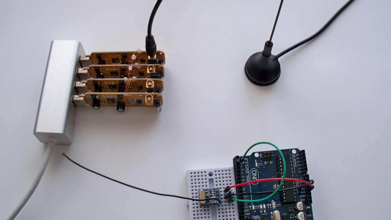
The Arduino generates data that is transmitted by the RF-module

The SDR reveices the signal, does some processing and passes the digitized signal to the PC

The SDR outputs two 8-bit unsigned values per sample, the real and the imaginary part of a complex number

The SDR was configured to record samples at a rate of 960kHz, meaning one sample every 1.04µs

The SDR was also configured to work at a center-frequency of 433.8MHz, meaning that a signal at 433.8MHz on air appears at 0Hz in the recorded file

The file below contains the raw samples as they were transmitted to the computer

18_sdr_uart_433.8MHz_960kHz.bin

The program below uses numpy to decode the data that was transmitted by the Arduino while plotting the signal at every processing step

1 baseband= samples * lo_sig
2 
3 plt.plot(abs(np.fft.fft(baseband[:2048])))
4 plt.show()

…

Save the code into the same directory as 18_sdr_uart_433.8MHz_960kHz.bin and run it

The following slides will guide you through the output of the program

1 plt.plot(abs(np.fft.fft(samples[:2048])))
2 plt.show()

To get an overview of an RF-signal it makes sense to look at it in the frequency-domain

To get from the time-domain (samples) to the frequency domain the fast fourier transform is applied to the first 2048 samples

The raw result of a fourier transformation has a few unintuitive properties:

• There are negative frequencies (this makes sense when working with complex-valued signals)
• The negative frequencies occur in the right half of the output (the output is often reorganized for visualization so that 0Hz is in the middle)

The plot above shows a peak at 130kHz

As the center frequency of the receiver was at 433.8Mhz this means, that the signal was originally sent at

433.8Mhz + 130kHz = 433.93MHz

For further analysis it makes sense to shift the signal to 0Hz, a process called mixing

1 offset_freq= -130e3
2 lo_sig= np.exp(2j * np.pi * offset_freq * t_hp)

To perform the mixing a signal with a frequency of -130kHz has to be generated (complex numbers are fun)

1 # Perform the shift
2 baseband= samples * lo_sig

The mixing is then performed by multiplying the receiver-signal with the generated signal

The signal is now centered at 0Hz

After mixing the signal to 0Hz we can filter away high frequencies and reduce the number of samples

1 lowpass= downsample(baseband)
2 sample_rate_lp= sample_rate / 100

The downsample function performs the filtering and keeps every 100th sample

1 abssig= abs(lowpass)
2 plt.plot(abssig)

After downsampling the signal is short enough to be displayed on screen

one can already start to see the UART-encoded data frames

To decode the frames one has to find the first sample below a certain threshold

afterwards the bits are decoded by slicing the frame into 10 symbols of equal length, according to the baudrate

if a bit is, on average, below the threshold it counts as 0, otherwise as a 1

1 >>> decoded_message= decode_message(
2 ...     abssig, 1200, 0.3)
3 ... )
4 >>> print('Message: {}'.format(decoded_message))
5 Message: Numpy + Matplotlib

When the last frame was processed the complete message is printed

Numpy ❤️ Matplotlib